Introduction: Why We Need LSM Trees Link to heading
Imagine you are managing a massive list of contacts.
- B-Trees are like a meticulously organized address book. Every contact has a fixed spot. Great for finding someone fast, but if you are constantly adding new contacts or updating addresses, you are always erasing, inserting, and reorganizing pages. This leads to slow, random writes.
- LSM Trees are different. New contacts go into a “new arrivals” pile in your hand (memory). When that pile gets big, you quickly write it down on a new sheet of paper (an immutable file) and add it to a stack of “recent additions.” Periodically, in the background, you merge these piles to remove duplicates and organize them. This makes adding new contacts incredibly fast, as you are mostly just appending.
This fundamental difference means LSM Trees are built for speedy writes, unlike B-Trees which prioritize reads.
Why B-Trees fall short for writes Link to heading
B-Trees struggle with write-heavy workloads because they perform in-place updates, leading to:
- Random disk writes: Slow, especially on HDDs.
- Page splits & double-writes: More I/O overhead.
- Write amplification: One logical write triggers multiple physical disk writes.
LSM Trees flip this by buffering writes in memory and deferring sorting/merging to background tasks. This results in:
- Fast sequential writes.
- Better compression.
- Tunable read/write trade-offs.
How LSM Trees Work (The Basics) Link to heading
- MemTable (In-Memory): All writes first hit this sorted memory buffer (often a skip list).
- WAL(Write-Ahead Log): Every write also appends to a disk-based log for crash recovery. If the system fails, we replay the WAL to restore the MemTable.
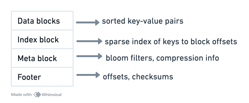
- SSTables (Immutable Sorted Files): When the MemTable fills, it’s flushed to disk as an SSTable. These files are always sorted and never modified. Each contains data blocks, an index, metadata (like Bloom filters), and a footer.
- Levels & Compaction: SSTables are organized into levels. Level 0 files (from MemTable flushes) can have overlapping keys. Higher levels (L1+) typically have non-overlapping, consolidated files.
- Compaction is a crucial background process that merges SSTables, discards obsolete data, and reduces read costs.
Compaction strategies Link to heading
- Size-Tiered (STCS): Merges similarly sized SSTables.
- Pros: Fast writes, less write amplification.
- Cons: Higher space usage, potentially slower reads (more files to check).
- Leveled (LCS): Merges SSTables from one level into the next, ensuring non-overlapping keys in higher levels.
- Pros: Lower read amplification, better space utilization.
- Cons: Higher write amplification (more data rewritten).
- Hybrid: Many systems use STCS for L0 (fast ingest) and LCS for higher levels (better reads).
How Reads Work Link to heading
Reads involve checking the MemTable, then Immutable MemTables, and finally iterating through SSTables from L0 upwards.
- Bloom filters quickly rule out SSTables that don’t contain the key, avoiding unnecessary disk I/O.
- A merge iterator combines results from all relevant sources, presenting the most recent version of a key.
- Block caches for hot data and key compression further optimize reads.
🧾 LSM vs. B-Tree: When to Use What Link to heading
| Feature | LSM Tree | B-Tree (e.g., InnoDB) |
|---|---|---|
| Writes | Sequential, fast, buffered | Random, in-place, can be slow |
| Reads | Slower (multiple lookups), optimized by cache | Fast, direct lookup |
| Compression | High (due to batching) | Lower |
| Write Amp. | Higher (due to compactions) | Lower |
Advanced Details & Tuning (very relevant to RocksDB) Link to heading
-
SSTable Indexing:
LSM Trees store data in immutable, sorted files called SSTables. To make reads efficient, even across large datasets and multiple levels, SSTables use:-
Sparse Indexing: Rather than indexing every key, SSTables store in-memory pointers to the start of each data block, allowing quick binary search and minimal memory usage. This lets the system jump directly to the relevant block on disk instead of scanning the whole file.
-
Key Prefix Compression: Since keys in sorted order tend to share common prefixes (e.g.,
user_123,user_124), SSTables compress keys by storing shared prefixes once per block and delta-encoding the rest. This reduces disk space and improves I/O performance.
-
-
Secondary Indexing in RocksDB: RocksDB doesn’t have native secondary indexes like relational databases. Instead, it’s typically implemented by creating separate column families (each an independent LSM Tree) that are sorted by the new secondary key. You would then query this “index” column family to find the primary key, then fetch the full record.
// Example: Writing to a secondary index column family in RocksDB using gorocksdb opts := gorocksdb.NewDefaultOptions() opts.SetCreateIfMissing(true) opts.SetCreateIfMissingColumnFamilies(true) dbPath := "/tmp/rocksdb-example" cfNames := []string{"default", "secondary_index"} cfOpts := []*gorocksdb.Options{opts, opts} db, cfHandles, err := gorocksdb.OpenDbColumnFamilies(opts, dbPath, cfNames, cfOpts) if err != nil { log.Fatal(err) } defer db.Close() defer cfHandles[0].Destroy() defer cfHandles[1].Destroy() wo := gorocksdb.NewDefaultWriteOptions() secondaryKey := fmt.Sprintf("username_idx:Alice:%d", userID) err = db.PutCF(wo, cfHandles[1], []byte(secondaryKey), []byte("user:123")) if err != nil { log.Fatal(err) } -
Time-Series Use Case: LSM Trees are ideal for time-ordered data due to efficient sequential writes and range deletes (via tombstones) for old data. Many time-series databases, including some built on concepts similar to RocksDB, leverage this.
-
Compaction Tuning (Common RocksDB parameters): Tuning compaction is crucial for performance.
max_background_compactions: Controls the number of parallel background compaction threads.level0_file_num_compaction_trigger: Number of L0 files that trigger compaction into L1.target_file_size_base: Influences the size of SSTables at different levels.- SSD vs. HDD: On SSDs, increase
max_subcompactions > 1for parallel compaction. On HDDs, keep compaction serialized to avoid “seek storms.”
-
Observability: Monitor
write_stall_micros(compaction backlog) andwrite_amplification(physical writes / logical writes) for performance debugging. Tools like RocksDB’sldb CLIand RocksDBExporter for Prometheus/Grafana provide vital insights.
When to Use LSM Trees Link to heading
- Your workload is write-heavy (logs, metrics, time-series, high-ingestion NoSQL).
- You can tolerate slightly higher read latency or have good caching.
- You are primarily using SSDs (they handle the random I/O from compaction better).
Avoid LSM Trees if:
- You need consistent, ultra-low-latency random reads (traditional OLTP).
- You are on HDDs with high write throughput (compaction can thrash disks).
References Link to heading
- CMU Database Systems Lecture: Storage II (LSM Trees)
- CMU Storage Lecture Notes (PDF)
- Key topics: LSM write path, compaction trade-offs, Bloom filters.
- Formal definitions of write amplification and LSM invariants.
- LSM Tree Visualizer on GitHub
- Interactive tool to observe MemTable flushes, SSTable levels, and compaction.
- ScyllaDB: What are SSTables?
- Production-grade SSTable implementation details (partitioning, compression).
- RocksDB Wiki
- Tuning guides, compaction algorithms, and API documentation.